4 LU Decomposition 4.1 Gaussian Elimination 4.3 Crout’s LU Factorization

4.2 Doolittle’s LU Factorization

An LU decomposition of A may be obtained by applying the definition of matrix multiplication to the equation A = LU. If $\mathbf{L}$ is unit lower triangular and U is upper triangular, then

$$a_{ij}=\displaystyle\sum_{p=1}^{\min(i,j)}l_{ip}u_{pj},\mbox{ where }1 \leq i,j \leq n$$

(45)

Rearranging the terms of Equation 45 yields

$$l_{ij}=\frac{a_{ij}-{\displaystyle\sum_{p=1}^{j-1}}l_{ip}u_{pj}}{u_{jj}},\mbox{ where }i \gt j$$

(46)

and

$$u_{ij}=a_{ij}-\displaystyle\sum_{p=1}^{i-1}l_{ip}u_{pj},\mbox{ where }1 \leq j$$

(47)

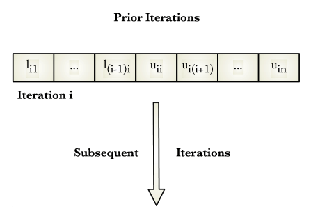
Jointly Equation 46 and Equation 47 are referred to as Doolittle’s method of computing the LU decomposition of A. Algorithm 2 implements Doolittle’s method. Calculations are sequenced to compute one row of L followed by the corresponding row of U until A is exhausted. You will observe that the procedure overwrites the subdiagonal portions of A with L and the upper triangular portions of A with U.

Algorithm 2: Doolittle’s LU Decompostion

for $i=1,\cdots,n$

for $j=1,\cdots,i-1$

$\alpha=a_{ij}$

for $p=1,\cdots,j-1$

$\alpha=\alpha-a_{ip}a_{pj}$

$a_{ij}=\displaystyle\frac{\alpha}{a_{jj}}$

for $j=i,\cdots,n$

$\alpha=a_{ij}$

for $p=1,\cdots,i-1$

$\alpha=\alpha-a_{ip}a_{pj}$

$a_{ij}=\alpha$

Figure 1 depicts the computational sequence associated with Doolittle’s method.

Figure 1: Computational Sequence of Doolittle’s Method

The computational sequence for used to create a LU factorization (decomposition) of a matrix using Doolittle's method

Two loops in the Doolittle algorithm are of the form

$$\alpha=\alpha-a_{ip}a_{pj}$$

(48)

These loops determine an element of the factorization l_ij or u_ij by computing the dot product of a partial column vector in U and partial row vector in L. As such, the loops perform an inner product accumulation.These computations have a numerical advantage over the gradual accumulation of l_ij or u_ij during each stage of Gaussian elimination (sometimes referred to as a partial sums accumulation). This advantage is based on the fact the product of two single precision floating point numbers is always computed with double precision arithmetic (at least in the C programming language). Because of this, the product a_ipa_pj suffers no loss of precision. If the product is accumulated in a double precision variable, $\alpha$ there is no loss of precision during the entire inner product calculation. Therefore, one double precision variable can preserve the numerical integrity of the inner product.

Recalling the partial sum accumulation loop of the elimination-based procedure,

$$a_{ij}=a_{ij}-\alpha w_{j}$$

You will observe that truncation to single precision must occur each time $a{}_{ij}$ is updated unless both A and w are stored in double precision arrays.

The derivation of Equation 46 and Equation 47 is discussed more fully in Conte and de Boor[5] .