2 Series Impedance 2 Series Impedance 2.2 Impedance of an N Conductor Transmission Line

2.1 Carson’s Equations

Carson’s formulas are

	$\displaystyle\mathbf{Z_{ii-g}}$	$\displaystyle=r_{i}+j2\omega ln\left(\frac{2h_{i}}{gm{r}_{i}}\right)+4\omega(P% +jQ)$		(1)
	$\displaystyle\mathbf{Z_{ij-g}}$	$\displaystyle=j2\omega ln\left(\frac{D_{ij}}{d_{ij}}\right)+4\omega(P+jQ)$		(2)

where

Z_ii–g is the self-impedance of conductor i with ground return.

Z_ij–g is the mutual impedance between conductors i and j with common ground return.

gmr_i is the effective radius (or geometric mean radius) of conductor i in centimeters.

h_i is the height of conductor i in centimeters.

r_i is the internal resistance of conductor i.

d_ij the distance between conductors i and j in centimeters.

D_ij the distance between conductor i and the image of conductor j in centimeters.

$\omega$ is 2 $\pi$ f, where f is the frequency in cycles per second.

Obviously, the self-impedance Z_ii–g and mutual impedance Z_ij–g can be decomposed into their real and imaginary components

	$\displaystyle\mathbf{Z_{ii-g}}$	$\displaystyle=R_{ii-g}+jX_{ii-g}$			(3)
	$\displaystyle\mathbf{Z_{ij-g}}$	$\displaystyle=R_{ij-g}+jX_{ij-g}$			(4)

Collecting terms in Equation 1 and Equation 2 and comparing to Equation 3 and Equation 4, it is apparent that

$\displaystyle R_{ii-g}$	$\displaystyle=r_{i}+4\omega P$	(5)
$\displaystyle R_{ij-g}$	$\displaystyle=4\omega P$	(6)
$\displaystyle X_{ii-g}$	$\displaystyle=2\omega ln\left(\frac{2h_{i}}{gm{r}_{j}}\right)+4\omega Q$	(7)
$\displaystyle X_{ij-g}$	$\displaystyle=2\omega ln\left(\frac{D_{ij}}{d_{ij}}\right)+4\omega Q$	(8)

2.1.1 Approximation of P and Q in Carson’s Equations

The P and Q terms in the preceding equations are defined by Carson as an infinite series expressed in terms of two parameters, call them k and $\theta$ . The form of P and Q are the same for Equation 1 and Equation 2. However, the value of k and $\theta$ differ. For self impedances

	$\displaystyle k$	$\displaystyle=4\pi{h}_{i}\sqrt{2\lambda f}$		(10)
	$\displaystyle\theta$	$\displaystyle=0$		(11)

For mutual impedances

	$\displaystyle k$	$\displaystyle=2\pi{D}_{ij}\sqrt{2\lambda f}$		(12)
	$\displaystyle\theta$	$\displaystyle=\frac{{cos}^{-1}({h}_{i}+{h}_{j})}{{D}_{ij}}$		(13)

where

$\lambda$ is the earth conductivity in ab℧/cm³.

$\theta$ is the angle defined in Figure 1.

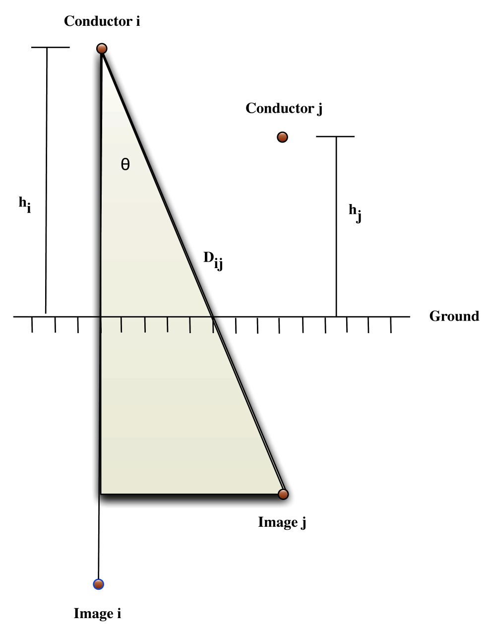
Figure 1: Transmission Line Geometry

Illustrates the geometry of an arbitrary overhead transmission transmission line configuration. Includes the dimensions and angles between conductors and their images required by Carson's equations.

Figure 1 defines the line geometry associated with Equation 10 through Equation 13.

The first few terms of the expansion of P and Q follow:

$\displaystyle P=$	$\displaystyle\frac{\pi}{8}-k\frac{\cos\theta}{3\sqrt{2}}+{k}^{2}\frac{\cos% \left(2\theta\right)\left(0.6728+\ln\left(\frac{2}{k}\right)\right)}{16}+{k}^{% 2}\frac{\theta\sin\left(2\theta\right)}{16}$	(14)
	$\displaystyle+{k}^{3}\frac{\cos\left(3\theta\right)}{45\sqrt{2}}-{k}^{4}\frac{% \pi\cos\left(4\theta\right)}{1536}$
$\displaystyle Q=$	$\displaystyle-0.0386+\frac{1}{2}ln\left(\frac{2}{k}\right)+k\frac{\cos\theta}{% 3\sqrt{2}}-\pi{k}^{2}\frac{\cos\left(2\theta\right)}{64}$	(15)
	$\displaystyle+{k}^{3}\frac{\cos\left(3\theta\right)}{45\sqrt{2}}-{k}^{4}\frac{% \sin\left(4\theta\right)}{384}-{k}^{4}\frac{\cos\left(4\theta\right)\left(1.08% 95+\ln\left(\frac{2}{k}\right)\right)}{384}$

2.1.2 Accuracy of Approximations to P and Q

Clarke (3) states that Equation 14 and Equation 15 exhibit less than one percent error for values of k up to one. Table 1 shows the wide applicability of these expressions for fundamental and harmonic analysis of power systems by examining values of k for a range of geometries, frequencies, and resistivities.

Table 1: Range of the Constant k

Distance	Frequency	Earth Resistivity	k
100 ft	60 Hz	10 Ω/m³	0.4196
	660 Hz		1.3916
	1020 Hz		1.7300

	60 Hz	100 Ω/m³	0.1327
	660 Hz		0.4401
	1020 Hz		0.5471

	60 Hz	1000 Ω/m³	0.0419
	660 Hz		0.1391
	1020 Hz		0.1730

100 ft - Large double circuit transmission tower
10 Ω/m ³ - Resistivity of swampy ground
100 Ω/m³ - Resistivity of average damp earth
1000 Ω/m³ - Resistivity of dry earth

2.1.3 Use of First Order Approximations to P and Q

At 60 Hz, it is common practice to ignore the higher order terms of the expansion of P and Q, i.e. let

	$\displaystyle P$	$\displaystyle=\frac{\pi}{8}$
	$\displaystyle Q$	$\displaystyle=-0.0386+\frac{1}{2}ln\left(\frac{2}{k}\right)$

This practice effectively decouples the series impedance from the conductor’s height above ground. According to Wagner and Evans (2), this omission tends to overstate the computed resistance and understate the computed reactance. At commercial frequencies and low earth resistivities ( $\rho$ =10), the first order approximations may introduce resistance errors in the neighborhood of 10 per cent. Under similar circumstances, self reactance errors rarely exceed one per cent. However, mutual reactance errors are more volatile. For $\rho$ =10, f=60, and D_ij=200 feet, the low order approximation of Q understates the mutual reactance by much as 4 per cent. At higher harmonics, these tendencies are magnified.